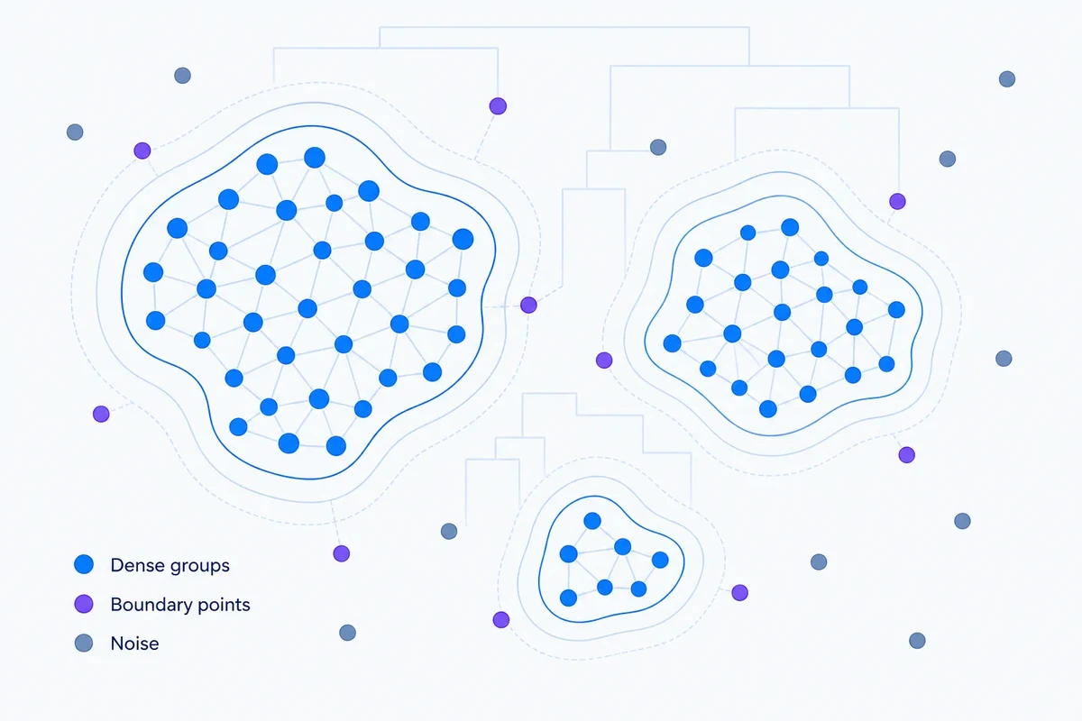
How to Cluster 100,000 Keywords Efficiently

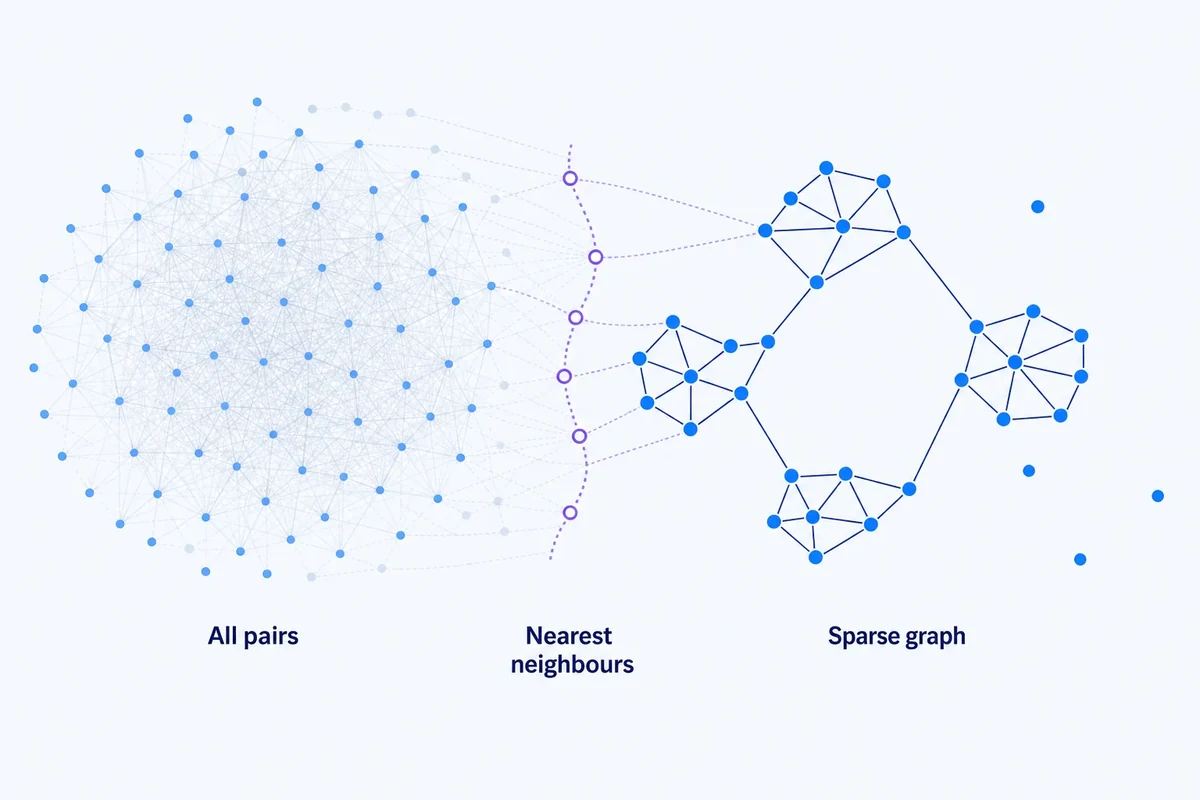
Most keyword research never gets anywhere near 100,000 rows. If you are working with 500, 2,000 or even 10,000 keywords, you can usually get a useful result without worrying too much about infrastructure.

At 100,000 keywords, that changes. The challenge is no longer just how to group the terms. It is how to avoid wasting time and memory comparing millions or billions of keyword pairs that could never be meaningfully related.

This is why large-scale clustering becomes an information-retrieval problem before it becomes a clustering problem.

The all-pairs problem

For n keywords, a naive undirected comparison considers roughly n(n-1)/2 pairs.

At 100,000 keywords, that means billions of potential relationships before you even begin clustering.

Most of them are useless. A query about enterprise CRM does not need to be compared exhaustively with every query about running shoes, shower trays and immigration law.

The first scaling decision is therefore not which clustering algorithm to use. It is how to reduce the number of candidate relationships without losing the ones that matter.

Separate embedding from neighbour discovery

A practical large-scale workflow has a few clear stages:

encode each keyword once;
store the resulting vectors;
retrieve a limited set of plausible neighbours for each vector;
keep or score the relationships that are actually useful;
cluster or build a graph from that much smaller relationship set.

That is very different from calculating a complete similarity matrix and then throwing most of it away.

Approximate nearest-neighbour search changes the economics

Libraries such as Faiss are designed for efficient similarity search over dense vectors. Instead of comparing every vector with every other vector, an index retrieves the most promising neighbours much more efficiently.

Approximate nearest-neighbour methods, often shortened to ANN, deliberately trade a small amount of retrieval accuracy for much larger gains in speed or memory.

For keyword clustering, that can be a sensible trade. You rarely need the exact ordering of every possible keyword pair. You need enough strong local relationships to recover the topical structure.

Do not confuse ANN recall with cluster quality

ANN is another modelling layer, so it needs its own checks.

If a genuinely related keyword is never retrieved as a candidate neighbour, the clustering stage cannot connect it later. That means ANN settings can change your final clusters even when the clustering algorithm itself stays exactly the same.

A useful QA process might:

sample pairs you already know should be related;
compare approximate retrieval with exact search on a smaller subset;
measure whether important neighbours are being missed;
check whether different ANN settings change graph connectivity or cluster stability.

The fastest index is not helpful if it drops the relationships that define your topics.

Sparse graphs are much easier to work with

Once every keyword keeps only its strongest neighbours, the dataset becomes a sparse graph rather than a dense similarity matrix.

That gives you several advantages:

lower memory usage;
fewer weak, irrelevant similarities;
a natural input for community-detection methods;
relationships that are easier to inspect;
a place to attach additional evidence to individual edges.

This is the same general idea explored in our keyword graphs article.

Top-k and threshold rules do different jobs

There are two common ways to keep that graph manageable.

Threshold rule: keep an edge only when similarity passes a chosen minimum.

Top-k rule: keep only the strongest k neighbours for each keyword.

A threshold protects relationship quality, but dense topics may still create lots of edges while unusual keywords become isolated.

Top-k gives you predictable graph size, but it can retain weak relationships simply because they are the best available for an odd query.

A hybrid is often more practical: retrieve the top candidate neighbours, then apply a minimum similarity rule and, where useful, a mutual-neighbour condition.

Our threshold-selection guide explains why that minimum should be tested against your own data rather than copied from someone else's setup.

Embed once and reuse the result

Embedding generation should be treated as reusable data rather than something you rerun every time you tweak a clustering parameter.

Store:

the keyword ID;
the exact text embedded;
model name and version;
vector dimensionality;
normalisation settings;
generation timestamp.

If the text and model have not changed, the vectors can usually be reused while you experiment with different graph or clustering settings.

This saves compute and makes comparisons between methods much cleaner.

Partitioning can help, but every partition is an assumption

You can also reduce the search space by splitting the dataset before neighbour discovery.

Possible partitions include:

language;
country;
brand;
high-level product family;
known business unit.

This can be very effective, but it comes with a cost. Once you divide the data, keywords on opposite sides of that boundary cannot discover each other.

Use partitions where the boundary is genuinely meaningful to the business, such as language or market. Avoid creating them purely because they make the computation easier.

Watch for giant connected components

A sparse graph can still become difficult to use if the edge rules are too generous.

Broad or generic terms can act as bridges and connect a large proportion of the dataset into one giant component. Community detection may still split that component, but the result can become unstable or hard to interpret.

Useful diagnostics include:

total edge count;
average degree;
percentage of isolated nodes;
connected-component sizes;
the largest component as a percentage of the graph;
cluster-size distribution.

These may look like engineering metrics, but they can have direct editorial consequences if they cause topics to merge or fragment in ways that make no sense to the user.

Memory matters as much as processing speed

Dense vectors can consume a lot of memory once you move into hundreds of thousands or millions of rows.

Practical options include:

using float32 where that precision is sufficient;
memory-mapped vector stores;
compressed or quantised ANN indexes;
processing sensible partitions in batches;
storing sparse edges rather than dense pair matrices.

Faiss includes index types that make different trade-offs between memory, speed and retrieval quality, including options that can use GPU hardware.

Scaling should not turn the workflow into a black box

When the dataset becomes too large to inspect row by row, explainability becomes more important, not less.

For any final cluster, you should still be able to inspect:

representative keywords;
nearest neighbours;
relationship strengths;
outliers;
the configuration used to create the graph;
why a particular keyword ended up where it did.

If you are presenting the output to a client, manager or content team, that traceability is what turns “the algorithm said so” into something people can actually trust and work with.

New keywords do not always require a complete rebuild

Suppose you have a 100,000-keyword dataset and add another 2,000 next month. Rebuilding every representation and relationship from scratch may be unnecessary.

The new keywords can be embedded and searched against the existing vector index. Depending on the method, they can either be assigned to the existing structure or held until a scheduled full rebuild.

The key distinction is between assignment and rediscovery. Assignment places new points into an existing model. Rediscovery allows the overall topic structure itself to change.

A practical architecture for 100,000 keywords

Clean and deduplicate conservatively. Remove true duplicates and obvious rubbish first.
Generate embeddings in batches. Cache them with model metadata.
Build an ANN index. Test retrieval quality on a known sample.
Retrieve plausible neighbours. Keep a manageable top-k candidate set.
Apply relationship rules. Use similarity floors, entities or other evidence where useful.
Build a sparse graph. Monitor density and connected components.
Run clustering or community analysis. Preserve confidence and noise rather than forcing everything into a group.
QA centres and boundaries. Do not review only the obvious keywords.

Engineering principle: scaling is not about making an all-pairs workflow run faster. It is about avoiding unnecessary comparisons while preserving the relationships you actually need.

ClusterIQ Conclusion

Most SEOs will never need to cluster 100,000 keywords in one job, and that is fine. The important lesson is that once the dataset becomes very large, the problem changes.

At that scale, dense all-pairs comparison wastes memory and compute on relationships that are almost certainly irrelevant. Approximate nearest-neighbour search, cached embeddings and sparse graphs make the workflow much more practical.

The trade-off is that retrieval settings become part of the analytical method. They need to be measured, versioned and checked, because performance optimisation should not quietly change the topical structure you are trying to understand.

Related ClusterIQ analysis

For retrieval infrastructure behind large corpora, see HNSW for SEO embeddings, Faiss index selection and ANN recall testing.

How to cluster 100,000 keywords without comparing every pair